In Class Ex 01

Author

Cheng Chun Chieh

Published

April 13, 2024

Modified

June 19, 2024

In Class Ex 01

1.1 Loading the required packages

pacman::p_load(tidyverse)

1.2 Loading the data

Rmb to use read_csv instead or read.csv

Using read_csv will retain the field names as per the csv file.

realis2019 <- read_csv("data/realis2019.csv")

2.1 Some Visualisation

First - to take a look at the data:

head(realis2019)

# A tibble: 6 × 20
  `Project Name`           Address    `No. of Units` `Area (sqm)` `Type of Area`
  <chr>                    <chr>               <dbl>        <dbl> <chr>         
1 PEIRCE VIEW              557 Upper…              1          113 Strata        
2 FLORIDA PARK             54 Sunris…              1          312 Land          
3 BULLION PARK             164 Lento…              1           75 Strata        
4 CASTLE GREEN             483 Yio C…              1          107 Strata        
5 HAPPY ESTATE             36 Thomso…              1          687 Land          
6 TEACHER'S HOUSING ESTATE 148 Tagor…              1          228 Land          
# ℹ 15 more variables: `Transacted Price ($)` <dbl>, `Nett Price($)` <chr>,
#   `Unit Price ($ psm)` <dbl>, `Unit Price ($ psf)` <dbl>, `Sale Date` <chr>,
#   `Property Type` <chr>, Tenure <chr>, `Completion Date` <chr>,
#   `Type of Sale` <chr>, `Purchaser Address Indicator` <chr>,
#   `Postal District` <dbl>, `Postal Sector` <dbl>, `Postal Code` <dbl>,
#   `Planning Region` <chr>, `Planning Area` <chr>

colnames(realis2019)

 [1] "Project Name"                "Address"                    
 [3] "No. of Units"                "Area (sqm)"                 
 [5] "Type of Area"                "Transacted Price ($)"       
 [7] "Nett Price($)"               "Unit Price ($ psm)"         
 [9] "Unit Price ($ psf)"          "Sale Date"                  
[11] "Property Type"               "Tenure"                     
[13] "Completion Date"             "Type of Sale"               
[15] "Purchaser Address Indicator" "Postal District"            
[17] "Postal Sector"               "Postal Code"                
[19] "Planning Region"             "Planning Area"

realis2019 <- realis2019 %>% 
  rename(
    unit_psm = 'Unit Price ($ psm)',
    unit_psf = 'Unit Price ($ psf)',
    sale_date = 'Sale Date',
    property_type = `Property Type`,
    sale_type = `Type of Sale`,
    planning_region = `Planning Region`,
    planning_area = `Planning Area`,
    trans_price = `Transacted Price ($)`
      )

Checking the transaction price across planning regions:

ggplot(data=realis2019, 
       aes(x= trans_price)) +
  geom_histogram(bins=50) +
  xlim (0, 5000000) +
  facet_wrap(~ planning_region) +
  labs(title="Histogram of Transacted Price across Planning Regions (up to $5M)", y="Count", x="Transacted Price ($)")+
  theme_minimal() +
  theme(axis.text.x = element_text(size = 6))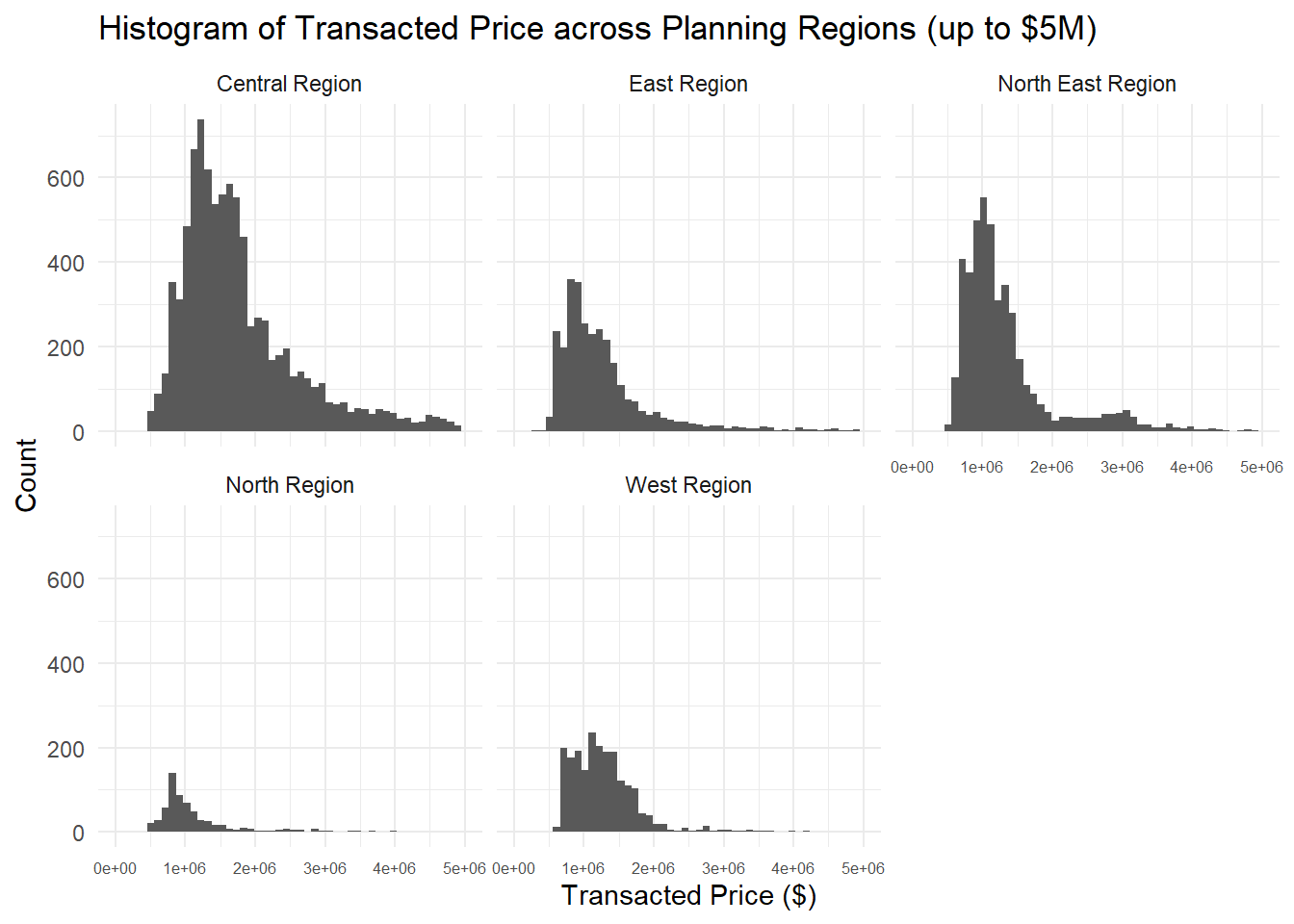

ggplot(data=realis2019, 
       aes(x= unit_psm)) +
  geom_histogram(bins=50) +
  labs(title="Histogram of Unit Price (psf)", y="Count", x="Transacted Price ($)") +
  theme_minimal()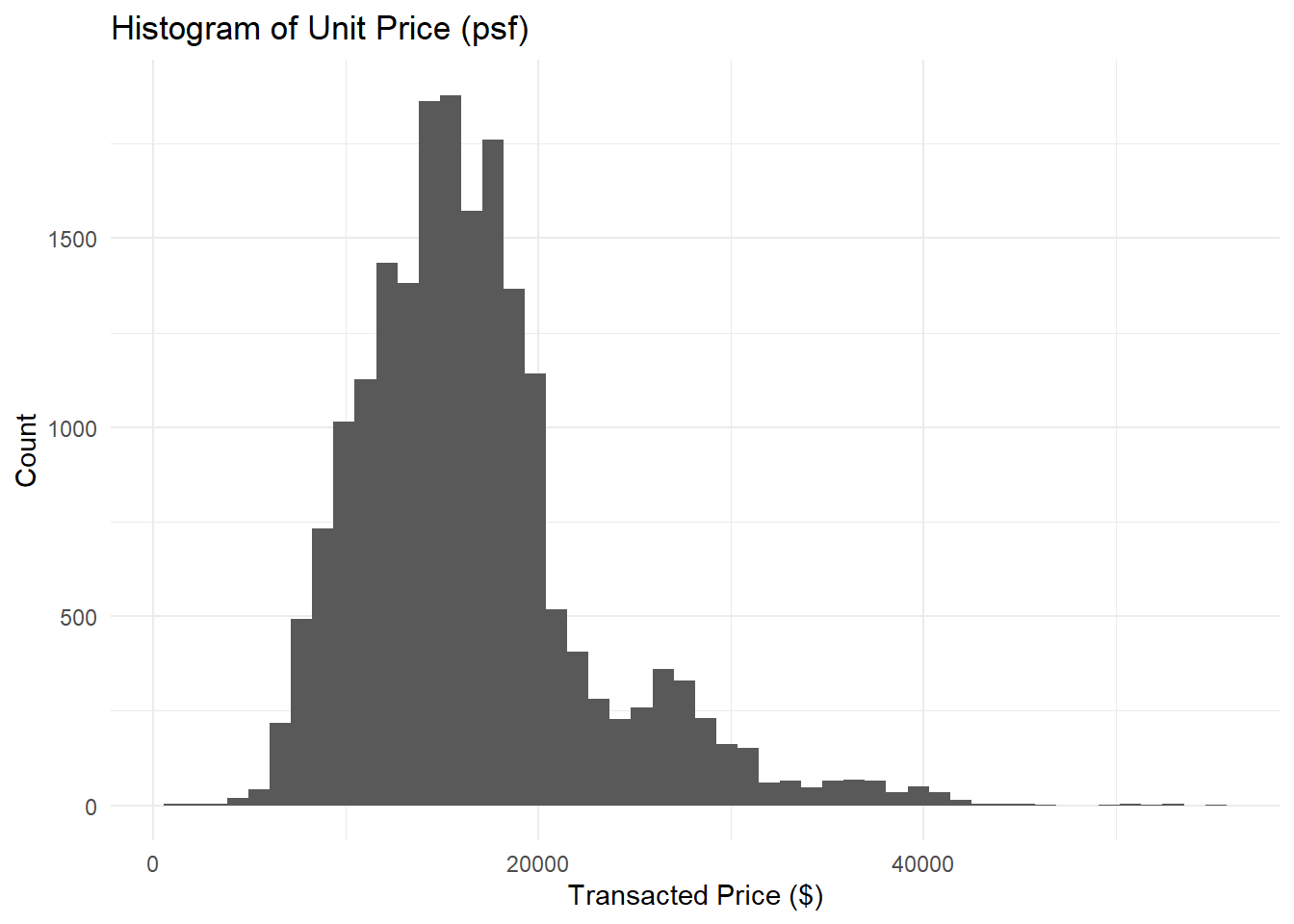

ggplot(data=realis2019, 
       aes(x= unit_psm)) +
  geom_histogram(bins=50) +
  facet_wrap(~ planning_region) +
  labs(title="Histogram of Unit Price (psf) across Planning Regions", y="Count", x="Transacted Price ($)")+
  theme_minimal() +
  theme(axis.text.x = element_text(size = 8))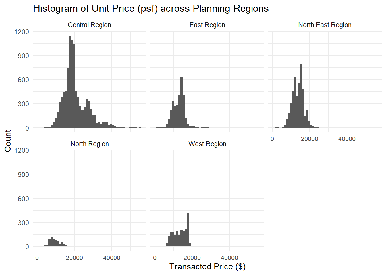

Taking a look at the unit price (psf) across property types:

ggplot(data=realis2019, 
       aes(y = unit_psf, x= property_type)) +
  geom_boxplot(colour ="black", fill="#88abff", alpha=0.5) +
  geom_point(stat="summary",        
             fun=mean,           
             colour ="darkblue",          
             size=2) +
  theme_light() +
  labs(title="Unit Price (psf) across Property Type", y="Unit Price ($psf)", x="Property Type")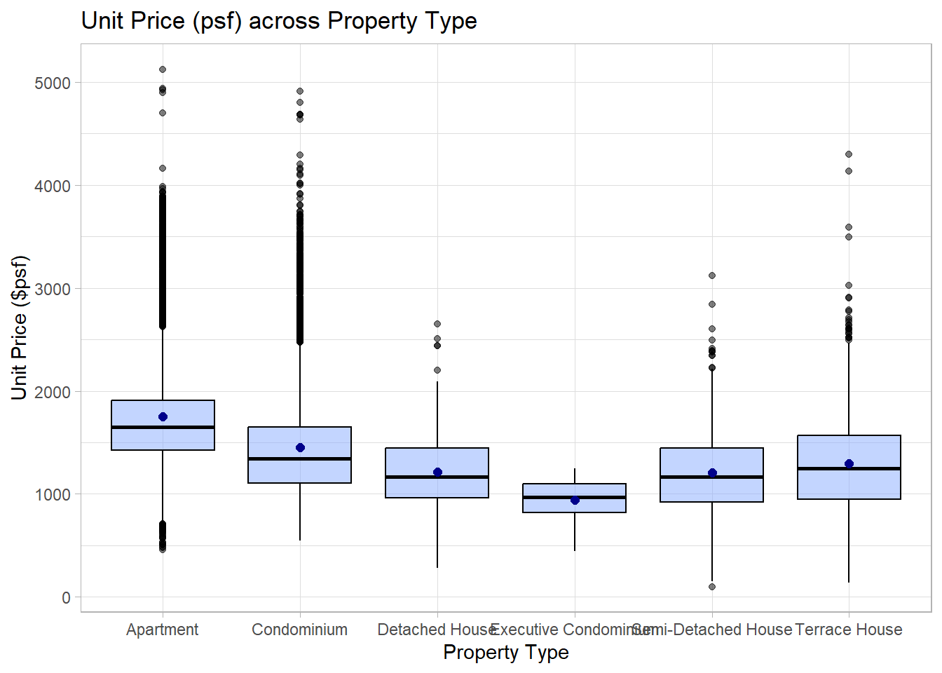

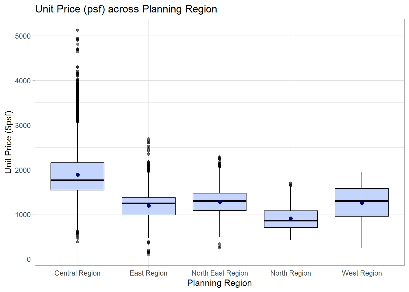
and across planning regions:

ggplot(data=realis2019, 
       aes(y = unit_psf, x= planning_region)) +
  geom_boxplot(colour ="black", fill="#88abff", alpha=0.5) +
  geom_point(stat="summary",        
             fun=mean,           
             colour ="darkblue",          
             size=2) +
  theme_light() +
  labs(title="Unit Price (psf) across Planning Region", y="Unit Price ($psf)", x="Planning Region")